Creating a sparse matrix

If a matrix A is stored in ordinary (dense) format, then the command S = sparse(A) creates a copy of the matrix stored in sparse format. For example:

>> A = [0 0 1;1 0 2;0 -3 0]
A =
     0     0     1
     1     0     2
     0    -3     0
>> S = sparse(A)
S =
   (2,1)        1
   (3,2)       -3
   (1,3)        1
   (2,3)        2
>> whos
  Name      Size         Bytes  Class

  A         3x3             72  double array
  S         3x3             64  sparse array

Grand total is 13 elements using 136 bytes

Unfortunately, this form of the sparse command is not particularly useful, since if A is large, it can be very time-consuming to first create it in dense format. The command S = sparse(m,n) creates an zero matrix in sparse format. Entries can then be added one-by-one:

>> A = sparse(3,2)
A =
   All zero sparse: 3-by-2
>> A(1,2)=1;
>> A(3,1)=4;
>> A(3,2)=-1;
>> A      
A =
   (3,1)        4
   (1,2)        1
   (3,2)       -1

(Of course, for this to be truly useful, the nonzeros would be added in a loop.)

Another version of the sparse command is S = sparse(I,J,S,m,n,maxnz). This creates an sparse matrix with entry (I(k),J(k)) equal to . The optional argument maxnz causes Matlab to pre-allocate storage for maxnz nonzero entries, which can increase efficiency in the case when more nonzeros will be added later to S.

There are still more versions of the sparse command. See help sparse for details.

The most common type of sparse matrix is a banded matrix, that is, a matrix with a few nonzero diagonals. Such a matrix can be created with the spdiags command. Consider the following matrix:

>> A
A =
    64   -16     0   -16     0     0     0     0     0
   -16    64   -16     0   -16     0     0     0     0
     0   -16    64     0     0   -16     0     0     0
   -16     0     0    64   -16     0   -16     0     0
     0   -16     0   -16    64   -16     0   -16     0
     0     0   -16     0   -16    64     0     0   -16
     0     0     0   -16     0     0    64   -16     0
     0     0     0     0   -16     0   -16    64   -16
     0     0     0     0     0   -16     0   -16    64

This is a matrix with 5 nonzero diagonals. In Matlab's indexing scheme, the nonzero diagonals of A are numbers -3, -1, 0, 1, and 3 (the main diagonal is number 0, the first subdiagonal is number -1, the first superdiagonal is number 1, and so forth). To create the same matrix in sparse format, it is first necessary to create a matrix containing the nonzero diagonals of A. Of course, the diagonals, regarded as column vectors, have different lengths; only the main diagonal has length 9. In order to gather the various diagonals in a single matrix, the shorter diagonals must be padded with zeros. The rule is that the extra zeros go at the bottom for subdiagonals and at the top for superdiagonals. Thus we create the following matrix:

>> B = [
   -16   -16    64     0     0
   -16   -16    64   -16     0
   -16     0    64   -16     0
   -16   -16    64     0   -16
   -16   -16    64   -16   -16
   -16     0    64   -16   -16
     0   -16    64     0   -16
     0   -16    64   -16   -16
     0     0    64   -16   -16
];

(notice the technique for entering the rows of a large matrix on several lines). The spdiags command also needs the indices of the diagonals:

>> d = [-3,-1,0,1,3];

The matrix is then created as follows:

S = spdiags(B,d,9,9);

The last two arguments give the size of S.

Perhaps the most common sparse matrix is the identity. Recall that an identity matrix can be created, in dense format, using the command eye. To create the identity matrix in sparse format, use I = speye(n).

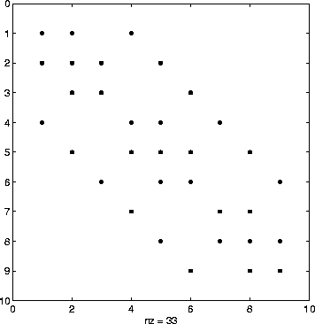
Another useful command is spy, which creates a graphic displaying the sparsity pattern of a matrix. For example, the above penta-diagonal matrix A can be displayed by the following command; see Figure 6:

>> spy(A)

  
Figure 6: The sparsity pattern of a matrix