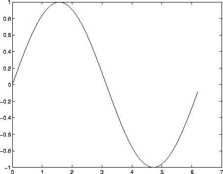
Figure 3: Graph of y = sin(x)
Matlab has many commands to create special matrices; the following command creates a row vector whose components increase arithmetically:
>> t = 1:5
t =
     1     2     3     4     5
The components can change by non-unit steps:
>> x = 0:.1:1
x =
  Columns 1 through 7
         0    0.1000    0.2000    0.3000    0.4000    0.5000    0.6000
  Columns 8 through 11
    0.7000    0.8000    0.9000    1.0000
A negative step is also allowed. The command linspace has similar
results; it creates a vector with linearly spaced entries. Specifically,
linspace(a,b,n) creates a vector of length n with entries
>> linspace(0,1,11)
ans =
  Columns 1 through 7
         0    0.1000    0.2000    0.3000    0.4000    0.5000    0.6000
  Columns 8 through 11
    0.7000    0.8000    0.9000    1.0000
There is a similar command logspace for creating vectors with
logarithmically spaced entries:
>> logspace(0,1,11)
ans =
  Columns 1 through 7
    1.0000    1.2589    1.5849    1.9953    2.5119    3.1623    3.9811
  Columns 8 through 11
    5.0119    6.3096    7.9433   10.0000
See help logspace for details.
A vector with linearly spaced entries can be regarded as defining a one-dimensional grid, which is useful for graphing functions. To create a graph of y = f(x) (or, to be precise, to graph points of the form (x,f(x)) and connect them with line segments), one can create a grid in the vector x and then create a vector y with the corresponding function values.
It is easy to create the needed vectors to graph a built-in function, since Matlab functions are vectorized. This means that if a built-in function such as sine is applied to a array, the effect is to create a new array of the same size whose entries are the function values of the entries of the original array. For example (see Figure 3):
>> x = (0:.1:2*pi);
>> y = sin(x);
>> plot(x,y)
Matlab also provides vectorized arithmetic operators, which are the same
as the ordinary operators, preceded by ``.''. For example, to graph
![]() :
:
>> x = (-5:.1:5);
>> y = x./(1+x.^2);
>> plot(x,y)
(the graph is not shown). Thus
x.^2 squares each component of x,
and x./z divides each component of x by the corresponding
component of z. Addition and subtraction are performed component-wise
by definition, so there are no ``.+'' or ``.-'' operators. Note the difference
between A^2 and A.^2. The first is only defined if
A is a square matrix, while the second is defined for any
n-dimensional array A.