STABILIZATION OF THE SPIKE POSITION (Jun 07, 2000)+(Jun 23, 2000)

Following Michael suggestion (though I haven't exhausted all the possibilities like varying just d₁ keeping d₂ fixed) I manage to stabilize (maybe) the steady state spike.

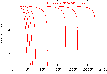
We take an initial spike centered at x=0 and our domain is taken to be [-1,1.5]. So the spike is closer to the x=-1 boundary. First let us look at the position of the spike as a function of time for different diffusive constants in the large range. In figure 8 we plot the position of the spike as time increases for d₁=d₂ ranging from 0.02 to 0.100 (right to left). In all these examples the spike travels towards its closest boundary with an increasing velocity.

  

Figure: Position of the spike as a function of time for large diffusion constants d₁=d₂.

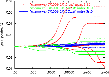
Now let us do the same for small diffusion constant. This is depicted by the red curves in figure 9 for which d₁=d₂ ranges from 0.001 to 0.015. As it is clear from this figure, the spikes do not travel towards the boundary. So we have stabilized the spike in a position different from the center or boundaries of the domain.

  

Figure: Position of the spike as a function of time for small diffusion constants d₁=d₂.

A very important and crucial point arises: is this phenomenon real or we are just watching an artifact of the numerics? The answer is provided by looking at the green and blue curves in the figure 9. For these new set of curves we introduce a better suited monitor function. Since it is very important to get the right `contact' between the tail of the spike and the boundary we need more mesh points near the boundaries. The new monitor function that we use for the green and blue set of curves leaves more points in the flat regions which in turn correspond to regions near the boundaries of the domain. For the green curves, as it can be noticed from the figure, the spikes stay closer to their initial position (x=0). This may indicate that indeed we are stabilizing the spikes. Moreover, if we increase the number of mesh points by a factor of two and keep the new monitor function it is possible to get an even better stabilization of the position of the spikes.

  

Figure: Snapshot of the stabilized spike for small diffusion constant ( d₁=d₁=0.008). Notice that the vertical axis is in logarithmic scale.

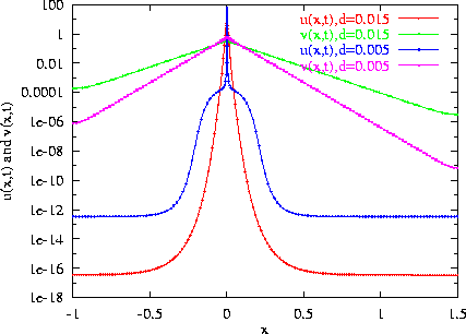This evidence would tend to suggest that if we use enough mesh points and a sophisticated enough monitor function for the mesh movement, the spikes may be pinned to their original positions. Another point that needs consideration is the fact that the spike may be pinned because the decay of its tail is so rapid that it does not manage to `feel' the boundary. In fact the spike in u(x,t) decays very rapidly and I believe that is not responsible for the movement of the spikes for larger diffusion. In figure 10 we plot a couple of snapshots of u(x,t) after the supposedly pinning. The red curve corresponds to d₁=d₂=0.15 and the blue curve corresponds to d₁=d₂=0.05. It is clear that the magnitude of u(x,t) near the boundaries is quite small. However, if we examine the v(x,t) variable we see a non-trivial tail that touches the boundaries (green curve for d₁=d₂=0.15 and pink curve for d₁=d₂=0.05).

Thus, if v(x,t) is the variable responsible for moving the center of the spike towards the boundary, we see from the figure that its magnitude is still quite considerable even for small d₁=d₂. This would stress the believe that the pining is a real effect and not just a numerical artifact.

MORE ABOUT PINNING (Jun 23, 2000)

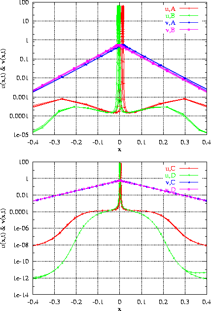
Re-taking the last idea we now show that it is u(x,t) and not v(x,t) (as indicated in the previous paragraph), who is responsible for the transient movement observed in figure 9. We also stress again the fact that the pinning of the spikes depends crucially on the monitor function.

In order to show that is u(x,t) and not v(x,t) the one responsible for the transient movement we plot in figure 11 the spike for different monitor functions. The monitor function is taken to be:

$$M = \sqrt{b+a_u u_{x}^2+a_v v_{x}^2+c_u u_{xx}^2+c_v v_{xx}^2}$$ (6)

where we vary the coefficients b,a_u,a_v,c_u,c_v to better suit the numerics. The coefficients give stress (i.e. put more grid points) to the following criteria:

- b: flat regions

- a_u|v: arclength of u(x,t)|v(x,t)

- c_u|v: curvature of u(x,t)|v(x,t)

We fixed the coefficients a=1 and c_u=c_v=0 and we varied the arclength coefficients a_u and a_v. The different plots (A to C) correspond to decreasing stress on arclength and increasing stress on flat regions. As it is observed from the figure, the shape of v(x,t) is independent from the choice of monitor function. However, the exact shape for u(x,t) depends crucially on the stress we put on flat regions. At the same time, the pinning of the spike requires the monitor function to give stress on the flat regions. This would tend to suggest that the transient movement of the spikes in figure 9 is due to a bad (too coarse) representation of the flat regions of u(x,t).

  

Figure: Profile of the spike for small d₁=d₂=0.005 for different monitor functions. The arclength coefficient correspond to A: a_u=0.1 and a_v=0.2, B: a_u=0.01 and a_v=0.02, C: a_u=0.001 and a_v=0.002 and D: a_u=0.0001 and a_v=0.0002.

From this last figure we can also infer that the pinning of the spike can be achieved by choosing a monitor function that gives enough stress to flat regions (i.e.  $a_u,a_v \ll b$). There is a very important question to ask at this point: is the pinned spike (for small enough a_u and a_v) going to travel eventually towards the boundary? I am currently running a few long-time computations to see if the spike eventually travels.

Another interesting point is to understand the shape of the actual solution for small diffusion constant. For this case, the spike seems to be constituted of two different scales: a wide base and a very narrow central peak (see figures 9 and 11).